Rolling Stock Analysis#
Introduction#
This tutorial explains the general workflow of running a rolling stock analysis. Based on two little examples we explain the necessary input for one load train with one velocity (example: tsi-beam-01.dat) and for multiple load trains and velocities (example: tsi-beam-02.dat).
Note
An advanced knowledge of the numerical input language CADINP and TEDDY is necessary to understand this tutorial.
Workflow#
For a rolling stock analysis special input is necessary in the following listed program modules:
PROG SOFiMSHA/C to define an edge or AXIS for the dynamic load application
PROG SOFiLOAD to define load trains
PROG DYNA for the dynamic analysis
PROG DYNR to plot the dynamic analysis results
Define an EDGE/AXIS#
Dynamic contact is governed by a changing location of contact point within time, as it is given in the case of a vehicle travelling along a bridge. It is mandatory to define a nodal sequense. There exist two options to define this nodal sequence:
use an EDGE from PROG SOFiMSHA
use a Structure Line from SOFiPLUS or SOFiMSHC
In both cases the database contains a list of nodes along the edge, no other data. Inside PROG SOFiMSHA the input looks like:
...
EDGE 1 FIT N1 1 N2 2 $ Generate a nodal sequence from node 1 to node 2
                     $ including all intermediate nodes
...
The number of this nodal sequence will be used later on in PROG DYNA command CONT. For additional visualisation an Axis can be used. We recommend that nodal sequence and axis are follw the same path. Please see alsoe the DYNA manual in chapter 3.14 ‘’CONT - Contact and Moving Load Function’’.
Define Load Trains#
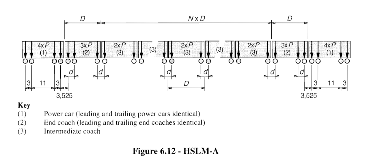
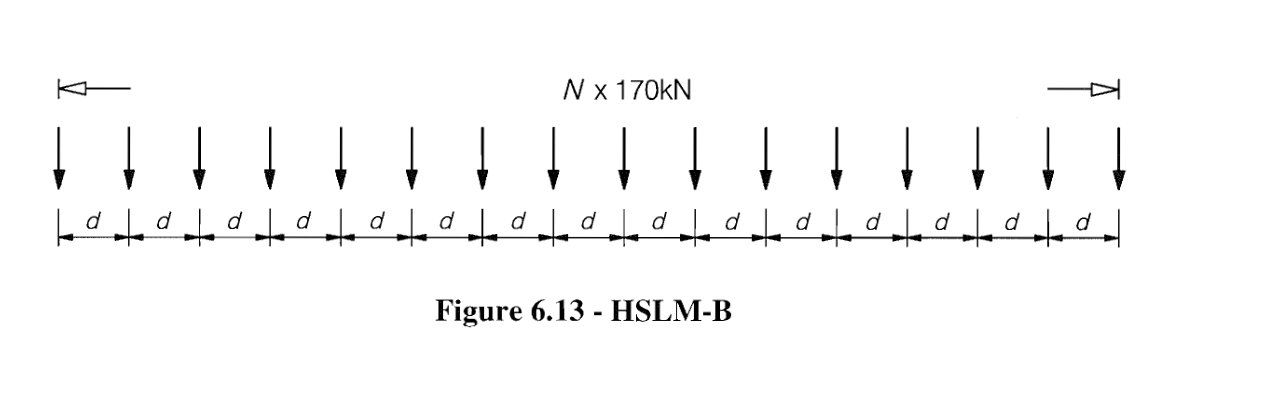
To define load trains we use the module SOFiLOAD and the record TRAI. For further description please see the SOFiLOAD manual chapter 5.5 “TRAI- Load Train Definition”. You may use predefined load trains as ICE3, TGV and others. The standard HSLM A and B load trains are available as well. If the load case has a load train created within SOFiLOAD, all loads of the train will follow each other with the appropriate distance.
Warning
Only point loads are processed by the CONT command.
The definitions are from EN 1991-2.
The general definition is a simple numerical input like:
LC 101 TYPE none titl 'Loadtrain HSLM A1'
TRAI HSLM P1 A1
There is also a nice little trick to define all 10 HSLM-A load trains within a loop including a variation of the load train class:
let#1 1
LOOP 10
 LC 100+#1 TITL 'Load Train' TYPE none
  TRAI TYPE HSLM P1 "A#1"
 let#1 #1+1
ENDLOOP
Start Dynamic Analysis#
For the dynamic analysis we will use some variables in order to have the same input for different project files. The variables will be defined and evaluated in a special module PROG TEMPLATE. Within the following input lines we use some special functions from the CADINP language:
+prog template
head  Definition of Analysis Parameters
let#xsi 0.05 $ Lehr's damping                           <-- manual input
let#f1 8     $ 1st Eigenform manual input necessary !!  <-- manual input
let#f2 45    $ 5th Eigenform                            <-- manual input
sto#a #xsi*4*3.1415*#f1/(#f1+#f2)
sto#b #xsi/3.1415/(#f1+#f2)

<TEXT> Damping

How to calculate Mass proportional damping and Stiffness proportional factor is
described  manual DYNA chapter 3.10.
The mean modal damping for concrete  ξ  = #(#xsi*100,3.0)%
The minimum frequency                f1 = #(#f1,3.0) Hz
The maximum frequency                f2 = #(#f2,3.0) Hz
Mass proportional damping factor      A = ξ*4π*f1*f2/(f1 + f2) = #(#a,13.6)
Stiffness proportional damping factor B = ξ/π/(f1 + f2)        = #(#b,13.6)

</TEXT>

LET#V 36                  $ SPEED in km/h               <-- manual input
sto#V #V/3.6              $ SPEED in m/sec from km/h
sto#lb 20                 $ length of bridge            <-- manual input
sto#lt 12                 $ lenght of load train        <-- manual input
sto#TT 1.5*(#lb+#lt)/#V   $ => total time is 1.5(lb..length bridge+lt..length load train)/#v
sto#STEP 0.10/20          $ time step lowest period/20  <-- manual input
<TEXT> Speed and Time Step

Speed of train passing         v = #(#v*3.6,10.2) km/h
Speed of train passing         v = #(#v,10.2) m/s
Length of bridge              lb = #(#lb,10.2) m
Length of load train          lt = #(#lt,10.2) m
Travelling time over bridge   tt = 1.5*(lb+lt)/v = #(#tt,10.2) s
Time step                   step = #(#step,10.5) s
</TEXT>
end
After all variable are known, we go for the dynamic analysis, which is a simple time step analysis taking into account the train passing. The necessary input for a single load train passing over the bridge with just one velocity looks like this:
+prog dyna
head Rolling Stock Analysis
CTRL RLC 10001                       $ save results for every single load step.
                                    $ Please use this option for small examples only!
STEP N #TT/#STEP DT #STEP A #a B #b  $ Time step integration
LC  103                              $ LOAD TRAIN ALONG EDGE 1 WITH AUTOMATIC TIME VALUES
CONT NR 1 V #V 0.0                   $ AUTOMATIC TIMEVALUES IN NODES FROM BEAMS
$
LET#LC 1000+101
HIST U-Z   1010 LCST  #LC  $ Save results for plots only
HIST A-Z   1010 LCST  #LC
HIST MY    1010 LCST  #LC

EXTR MY MAX 101 MIN 102               $ Save results in data base
END
Example 1#
Note
This example shows the general workflow described above on a single span bridge with one load train and one velocity.
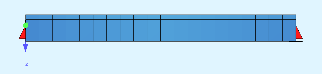
The first example is a single beam bridge with a span of L = 20 m.
As a load we apply a user defined load train:
LC 103 type none titl 'User Loadtrain'
trai user        $ total lenth = 12.0 m
trpl P 100
trpl p 100 a -2
trpl p 100 a -8
trpl p 100 a -2
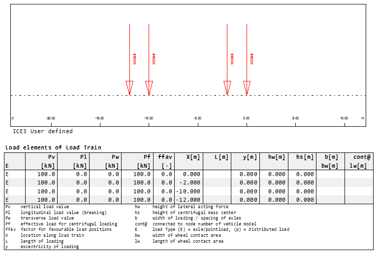
The user defined load train has a passing velocity of 36 km/h = 10 m/s. The next picture shows the beam moment MY for the static train load in midspan of the bridge compared to the dynamic results.

Example 2#
Note
This example shows the general workflow described above on a single span bridge with multiple load trains and velocities.
This example is nearly the same as example 1, except the following difference:
instead of a user defined load train we will use all 10 HSLM-A load trains
instead of only one velocity we apply the loads for velocities from 120 km/h to 360 km/h with an increment of 10 km/h
The input is slightly different. First of all we must generate the necessary variables and velocities in a module TEMPLATE:
+prog template
head  Definition of Analysis Parameters
let#xsi 0.05  $ Lehr's damping
let#f1 8      $ 1st Eigenform  manual input necessary !!
let#f2 45     $ 5th Eigenform
sto#a 4*3.1415*#f1/(#f1+#f2)
sto#b #xsi/3.1415/(#f1+#f2)
<TEXT> Damping
How to calculate Mass proportional damping and Stiffness proportional factor is
described  manual DYNA chapter 3.10.
The mean modal damping for concrete  ξ  = #(#xsi*100,3.0)%
The minimum frequency                f1 = #(#f1,3.0) Hz
The maximum frequency                f2 = #(#f2,3.0) Hz
Mass proportional damping factor       A = ξ*4π*f1*f2/(f1 + f2) = #(#a,13.6)
Stiffness proportional damping factor B = ξ/π/(f1 + f2)        = #(#b,13.6)
</TEXT>
$ Values of Speedparameter
sto#SPEEDPAR 120,360,10 $ min. speed, max. speed ,increment
loop#speed  (#SPEEDPAR(1)-#SPEEDPAR(0))/#SPEEDPAR(2)+1
LET#V1 #SPEEDPAR(0)+#SPEED*#SPEEDPAR(2) $ SPEED in km/h
LET#V #V1/3.6                           $ SPEED in m/sec from km/h
sto#lb 20                 $ length of bridge
sto#lt 400                $ length of load train
LET#TT 1.5*(#lb+#lt)/#V   $ => total time is 1.5(lb..length bridge+lt..length load train)/#v
sto#STEP 0.10/20          $ time step lowest period/20
<TEXT> <U>Variable Time Step Analysis #(#speed+1,2)</U>
Speed of train passing         v = #(#v*3.6,10.2) km/h
Speed of train passing         v = #(#v,10.2) m/s
Travelling time over bridge   tt = 1.5*(lb+lt)/v = #(#tt,10.2) s
Length of bridge              lb = #(#lb,10.2) m
Length of load train          lt = #(#lt,10.2) m
Time step                   step = #(#step,10.5) s
</TEXT>
endloop
end
Similar changes must be made in the module DYNA:
+prog dyna
head DYNAMIC PASSING OF LOADS OF TRAINS
LOOP#TRAIN 10  $ HSLM A1 - A10
LOOP#SPEED (#SPEEDPAR(1)-#SPEEDPAR(0))/#SPEEDPAR(2)+1
   ctrl solv 3
   LET#V1 #SPEEDPAR(0)+#SPEED*#SPEEDPAR(2) $ SPEED in km/h
   LET#V #V1/3.6                           $ SPEED in m/sec from km/h
   LET#TT 1.5*(#lb+#lt)/#V                 $ total travelling time
$ process analysis
   STEP N #TT/#STEP DT #STEP A #a B #b $ Time step integration
   LC  101+#TRAIN         $ LOAD TRAIN ALONG EDGE 1 WITH AUTOMATIC TIME VALUES
   CONT NR 1 V #V YEX 0.0 $ AUTOMATIC TIMEVALUES IN NODES FROM BEAMS
$ Save results for plots
   LET#LC 1000+100*#TRAIN+2*#SPEED
   #define LC1=#LC
   HIST U-Z   1010 LCST  #LC
   HIST A-Z   1010 LCST  #LC
   HIST MY    1010 LCST  #LC
$ save results in database
   extr u  max #lc min #lc+1 ACT L
   extr a  max #lc min #lc+1 ACT L
   extr MY max #lc min #lc+1 ACT L
   END
ENDLOOP
ENDLOOP
END
The basic idea behind the two loops is to have
a loop for the different load trains and
a loop over all velocities.
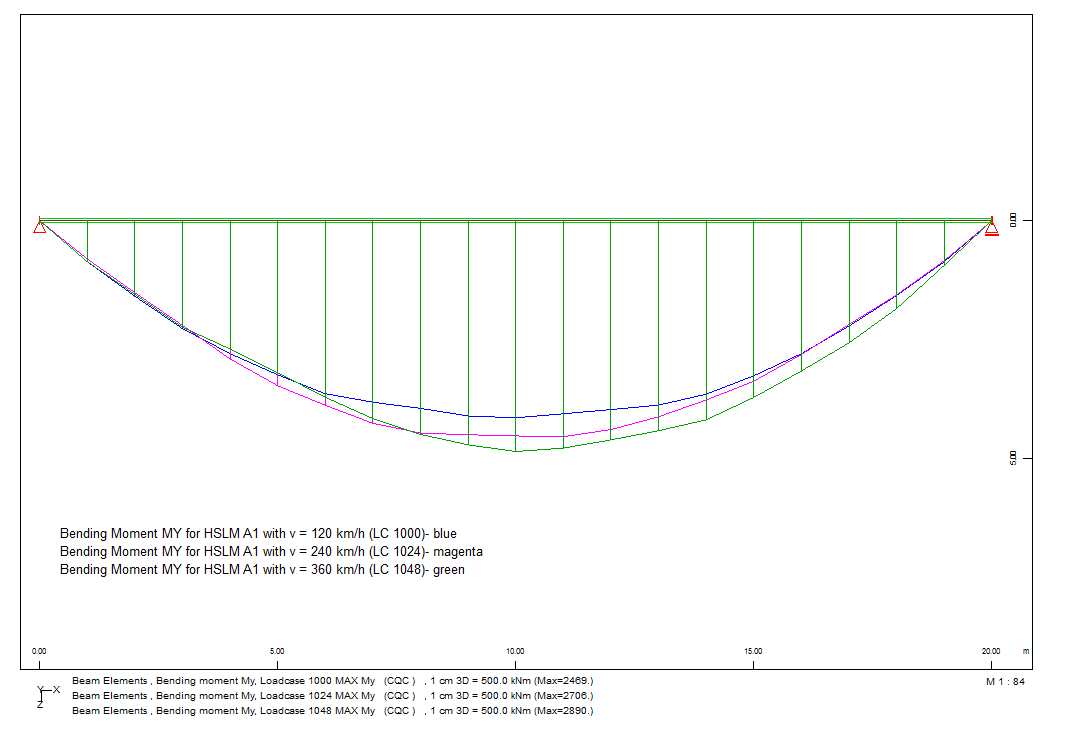
The results are shown in the picture below:
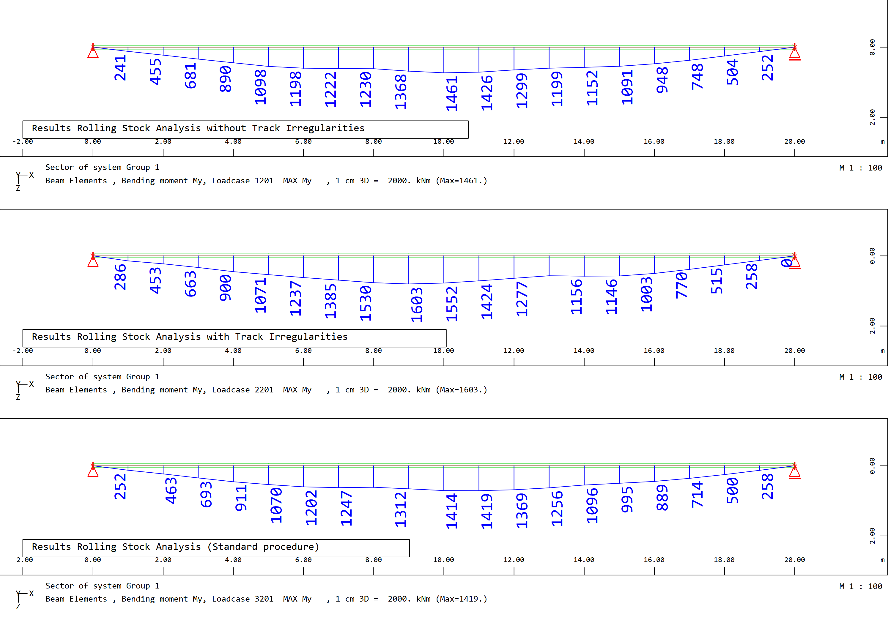
Example 3#
Note
This complex example deals with the problem of simulation a rolling stock with a real train system, containing wheel and bogi. Additional track irregularities will be used inside this example as well. Inside this example we compare the results with and without track irregularities.
Finally we want to model a bridge with a real train passing over. The train is modelled with a beam structure supported with a spring damper system at the beginning and the end of vehicle. The beam elements are without any mass. The total mass of this vehicle is applied in the centre with a specific value. Please see the input as follows:
+prog sofimsha  $Train FE-Model
head Train FE-Model
syst rest  gdiv 1000   gdir posz  $ add new elements to system
ctrl rest 2                       $ don't delete already existing loads loads

$   System Train Structure
$
$
$   1022             1030              1012
$    x-----------------x-----------------x
$    /             Mz=#Mv                /
$    \            myy=#Iv                \ Spring+Damper
$    /                                   /
$    \                                   \
$    x                                   x
$   1021                               1011
$
node 1011 x -1.0  0.0  0.0
node 1012 x -1.0  0.0 -1.0
node 1021,1022 x -#Lc      nr1 1011,1012
node 1030      x -0.5*#Lc  nr1 1012

grp 2
beam no 1 na 1022 ne 1030 ncs #t_sno
beam no 2 na 1030 ne 1012 ncs #t_sno
spri no 1 na 1011 ne 1012 dz 1.0 cp #kv dp #cv
spri no 2 na 1021 ne 1022 dz 1.0 cp #kv dp #cv
mass no 1030 mz #Mv myy #Iv
$ constraints:
$ 1) no displacement in y-direction
$ 2) no torsional rotation of the vehicle
$ 3) horizontal displacement of a wheel = top of a vehicle
node      1011,1021 fix py
node 1030,1012,1022 fix pymx
kine nd 1011 fix px nd1 1012 fd1 1
kine nd 1021 fix px nd1 1022 fd1 1
end
To make sure the program will use this vehicle definition we must connect our user defined load train with the connection nodes of the vehicle. This will be done within the definition of the load train in PROG SOFiLOAD:
+prog sofiload $Vehicle definition
head  Vehicle definition
$ suspended rigid bar
lc 101 titl 'Vehicle'
trai user
trpl p 0.5*#Mv*9.81 a   -0 cont  1011  $ force = mass*g, contact node = 1011
trpl p 0.5*#Mv*9.81 a -#Lc cont  1021  $ force = mass*g, contact node = 1021
end
The general procedure of the time step analysis is the same as in the previous examples. The track irregularities will be applied with additional functions. There are three main functions possible. All functions are set inside the STEP record in PROG DYNA with:
vertical track irregularities STEP … LCUV
transverse track irregularities STEP … LCUT
rotational track irregularities STEP …LCUR
The basic idea is to generate artificial track irregularities based on an intensity function and a power spectra using the SIMQ procedure. In the following example we follow the functions published by the ORE in 1989. Please read the additional comments inside the example input file. The time step analysis follows the general input including the information about the track irregularities.
STEP N #TT/#STEP DT #STEP THE 0.7    $ Time step integration
LC  102                              $ LOAD TRAIN ALONG EDGE 1 WITH AUTOMATIC TIME VALUES
CONT NR 1 V #V 0.0                   $ AUTOMATIC TIMEVALUES IN NODES FROM BEAMS
Please see the comparison of beam bending moments MY for a rolling stock with real vehicle simulation, without and with track irregularities and a standard rolling stock analysis with a user defined load train.