Dynamic Analysis - Moving Load Trains#
Introduction#
Welcome to the Dynamic Analysis - Moving Loads Trains tutorial.
In this tutorial we show the workflow for the dynamic analysis of railway bridges under moving loads, like for example described in EN 1991-2, section 6.4.6 or UIC CODE 776-2, section A.6.1.
We demonstrate the workflow on a simple single span concrete beam bridge.
We show how to calculate eigenfrequencies and display the mode shapes of the structure.
We explain how to define the load models (“load trains”) for the train passages.
To show the basic workflow we explain how to calculate a single passage for one of the defined load trains. Here we also show how you can determine a reasonable timestep size for the analysis by using an automatic convergence study.
Usually the analysis has to be performed not only for a single train type with one certain speed, but for many passages with different train types and speeds. The next step of the tutorial explains how to efficiently set up these calculations.
As final point we show the postprocessing options to display and document the calculated results.
By the end of the tutorial, you should be able to:
Calculate eigenfrequencies and mode shapes of your structure
Define the load trains for the analysis
Conduct a dynamic analysis for one or many train passages
Postprocess the results (i.e. plot time histories, calculate a dynamic amplification factor, generate result envelopes, determine resonance velocities for different train types)
Project Description#
In this tutorial we investigate a simple concrete beam bridge with a span length of 20m.
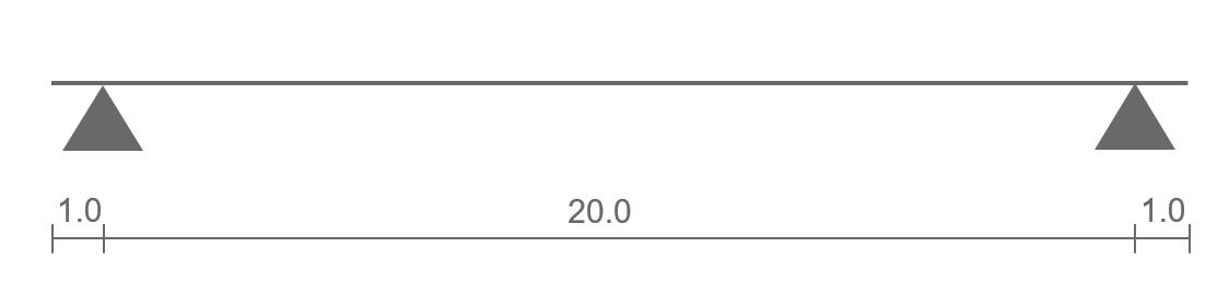
System
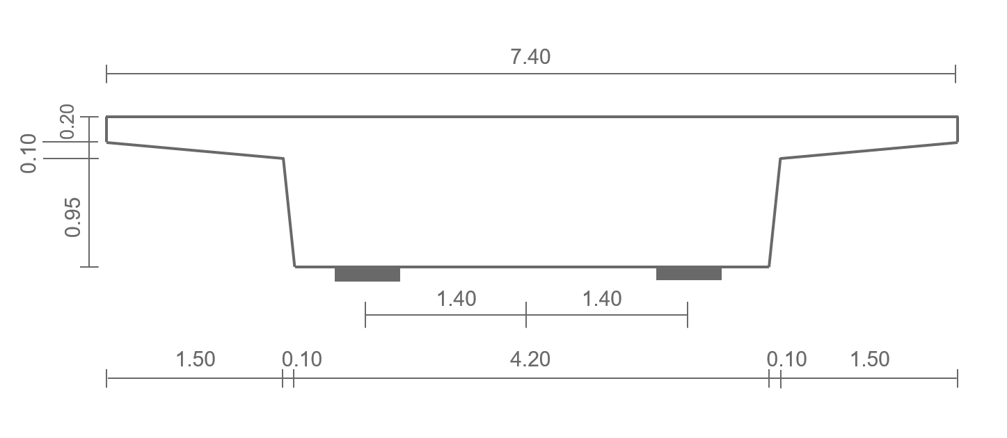
Bridge cross-section
System Generation#
In the following video we show you how to create the bridge model for this tutorial using our parametric, axis based modelling concept CABD.
Dynamic Eigenmode Analysis#
As starting point for the analysis we would like to know the eigenfrequencies and corresponding mode shapes of the structure. For this purpose we do a dynamic eigenmode analysis using the corresponding task.
Load Train Definition#
In order to calculate the train passages we first have to define the load models for the trains types that we want to investigate. In the follwing video we show you how to do it.
Dynamic Analysis - Basic example#
To introduce the setup of the dynamic analysis we will first calculate the passage of one train with one velocity. Based on this setup, we will then in the next section explain how to efficiently set up the analysis for all trains and all velocities.

Dynamic Analysis for all trains and all speeds#
After having introduced the general setup of for the dynamic analysis we show how to efficiently set up the calculation for all trains of interest and for the complete velocity range.

Postprocessing#
After having calculated all train passages we can postprocess and plot the results. We explain how to plot time histories, calculate a dynamic amplification factor and create a result envelope containing the extremal results of all train passages. Finally we show you how to create a graph displaying the development of a selected result over the velocity range for the individual train types to detect resonance velocities for the different train types. For the postprocessing we use our standard tools such as Graphic and Result Viewer.
