Special vehicles (LM3) with Traffic Loader#
General information#
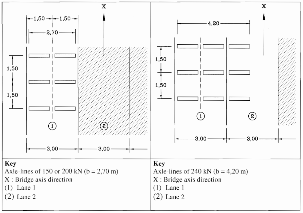
In Annex A of EN 1991-2 there are several types of special vehicles defined for the application on road bridges.
They can be distinguished in vehicles with two wheels per axle (axle loads of 150 kN or 200 kN) and three wheels per axle (axle load of 240 kN).
According EN 1991-2 the special vehicle usually does not act alone, but is applied in combination with the frequent values of the loads from the standard load model LM1.
In the following sections, we show you how to use the different special vehicles within the traffic loader and how to take into account the LM1.
Note
If and how to apply special vehicles (LM3) is usually determined by the national annex relevant for your project. In this tutorial we show the most important settings based on general examples. Adjust them for the requirements of your individual project!
Special vehicles with axle loads of 150 kN or 200 kN#
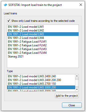
In this tutorial we will apply LM3 3000 200 (see EN 1991-2, table A1) in the Traffic Loader. We recommend to add a new Traffic Loader task to your project for the analysis of special vehicles. We will show you step by step the most important settings in the tabs of the task.
Load trains#
We want to have the standard load model LM1 to act togehter with the special vehicle. For this purpose we first define the necessary LM1 load trains as usual.
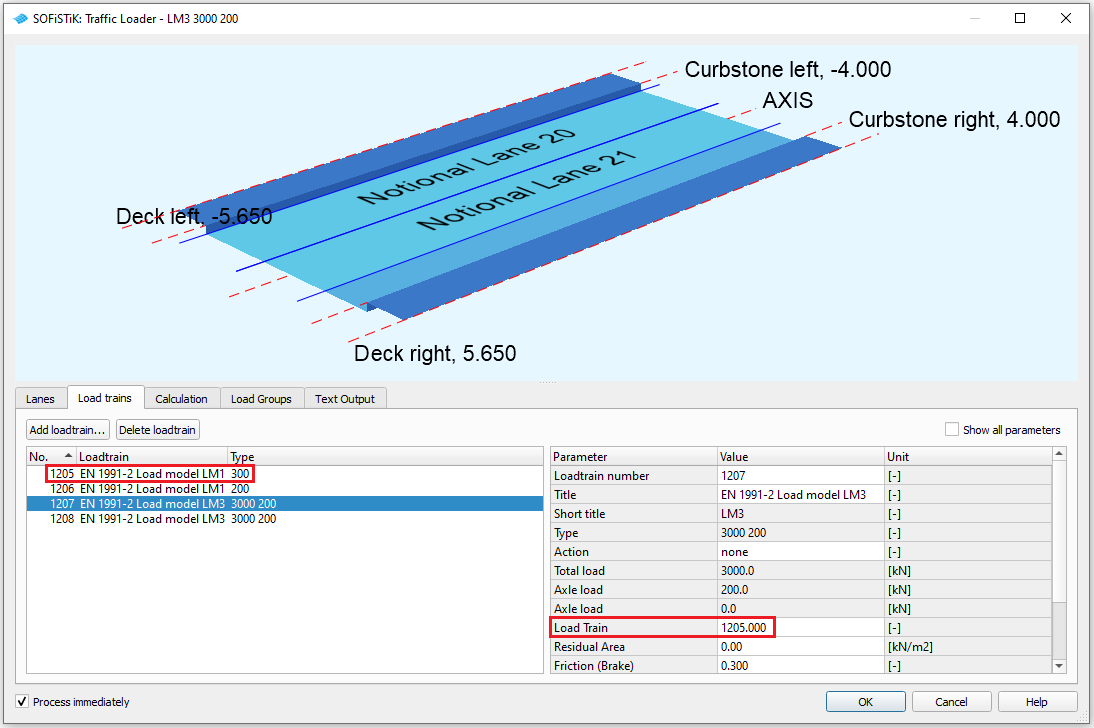
Next we define the special vehicle. Click on the Add loadtrain button. Select EN 1991-2 Load model LM3 3000 200 and add it.
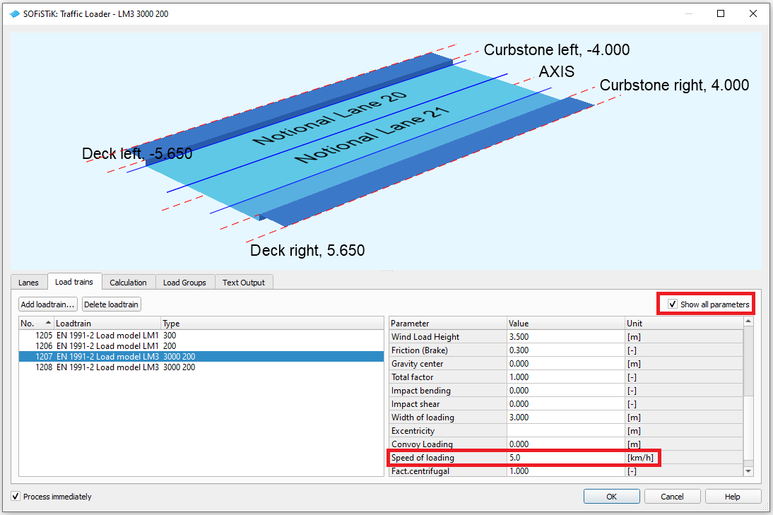
Depending on the speed of the load train a dynamic amplification factor is applied (see also EN 1991-2 A.3). Set a low speed (5 km/h) for the load train, if you don’t want a dynamic amplification to be used.
Next we define that the special vehicle should be accommpanied with the LM1. This is done via the option Load Train. Set the number of the accompanying LM1 here.
Note
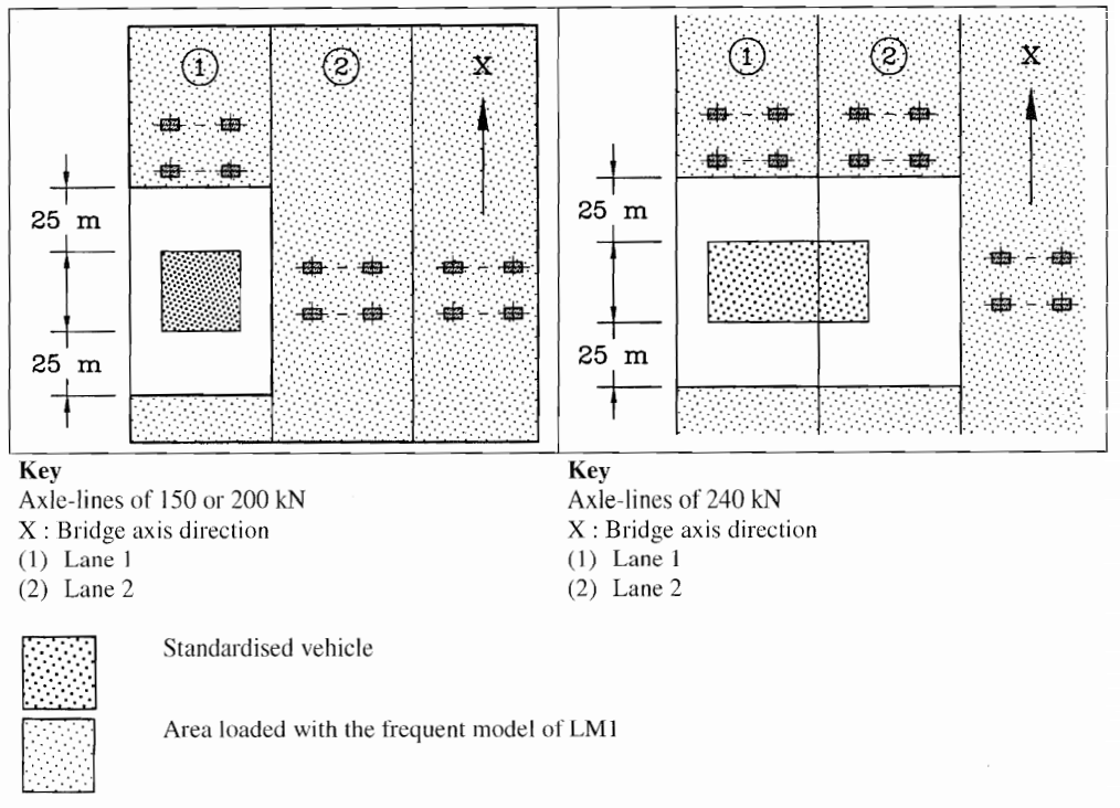
The specification from EN 1991-2, that no additional load should be applied within a distance of 25 m to the special vehicle is considered automatically.
Important
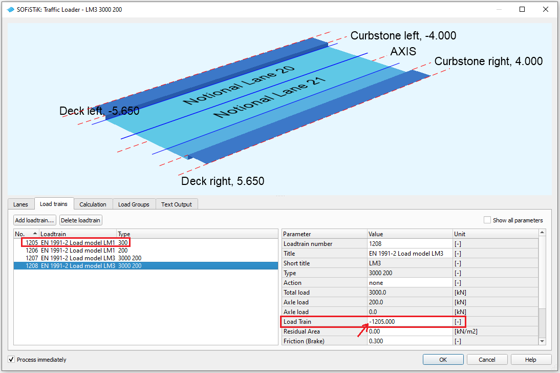
The program can not decide by itself, if the tandem axis of the LM1 should be placed before or after the LM3. This has to be defined by the user. Specifying the acommpanying load train without (resp. with positive) sign means the tandem axis is placed in front of the special vehicle. If you add the acommpanying load train with negative sign, it is following the special vehicle. For a detailed investigation it can be necessary to define the LM3 twice: once with positive sign and once with negative sign for the accompanying LM1.
Calculation#
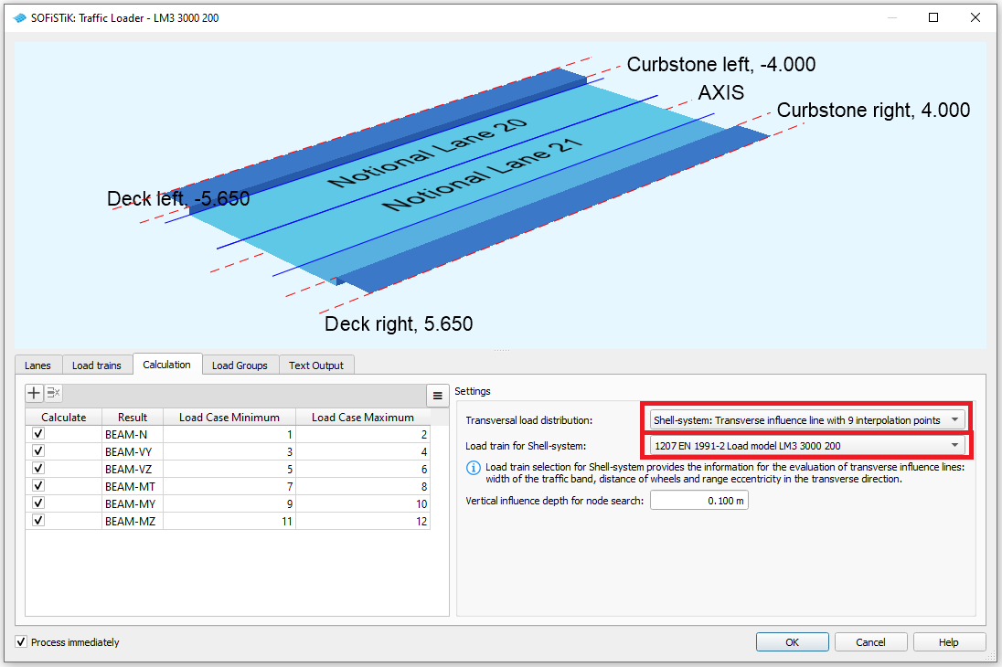
In this tutorial we have a hybrid system including shell elements. For such a system it is mandatory for the calculation to evaluate transverse influence lines to determine the load distribution in cross-direction. For the correct evaluation of the transverse influence line the information about the geometry of the load train (esp. its width and the wheel spacing in cross-direction) is important. Therefore we have to specify the load train for the evaluation. Set one of the defined LM3 load trains. They have the information about their own wheel spacing (1.5 m) and the wheel spacing of the LM1 tandem axis (2.0 m), thus enabling a correct calculation for both load train types.
Note
This specification is not necessary, if a load distribution for single or multi girder systems (i.e. pure beam systems) has been chosen.
Load Groups#
Finally we define the load group(s) for the evaluation.
Note
Make sure to choose an appropriate action for the superpositioning of the final design envelopes. This action has already to be defined within the Action Manager.
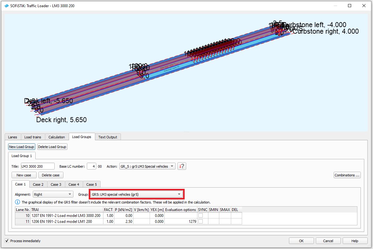
Add Cases to the load group for the scenarios you want to investigate.
Select in the Group selection GR5: LM3 special vehicles (gr5). With this setting the loads from LM1 will be applied with their frequent values (acc. EN 1991-2 A.3).
Set the LM3 load train (with accompaying LM1) in the lane you want to place it.
Add additional (LM1) load trains in other lanes if necessary.
For example in Case 1 in the following picture we have applied the special vehicle with acommpanying LM1 (frequent values of: TS with axle load 300 kN; UDL loads of 9kN/m2) in lane 10 (most right aligned). In lane 11 we have additionally applied the second LM1 load train (frequent values of: TS with axle load 200 kN; UDL loads of 2.5kN/m2).
Important
Remember that the LM1 can be defined to be in front of or following the special vehicle. It may be necessary to investigate several cases with different load train definitions to find the decisive load position for each element.
Note
In the visualization window of the task you get an schematic overview, how the load trains are applied. This view is only available, if the used load trains are already saved in the database (i.e. after you have calculated the task for the first time). The LM1 load trains are always depicted with characteristic loads in the visualization, even if the frequent values are applied with Group selection GR5: LM3 special vehicles (gr5).
Text Output#
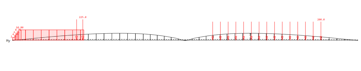
We recommend to check the calculation also by taking a look at some of the created influence lines.
You can add a new sequence of influence line plots by clicking on the New button and graphically select an element in the System Visualization with the ![]() button.
button.
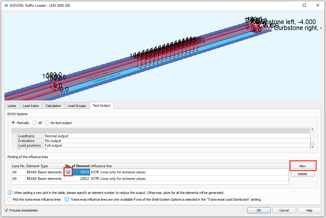
By checking the influence lines in the report you can see the decisive load position within each of the selected axes for the selected element and force component.
Special vehicles with axle load of 240 kN#
These load models usually do not fit within a single lane
Because loads that go beyond the borders of a lane are clipped (i.e. not applied) in the analysis, we need a special setting for these load trains.
We will show this at the example of the special vehicle LM3 3600 240
The settings in the Load Train and Calculation tabs are analog to those for the special vehicles with 2 wheels per axle. Select the load trains and specify acommpanying load trains and speed of the vehicle and make the adjustments for the calculation of the transverse influence lines.
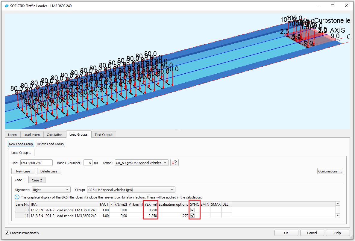
The important adjustment comes in the Load Groups tab:
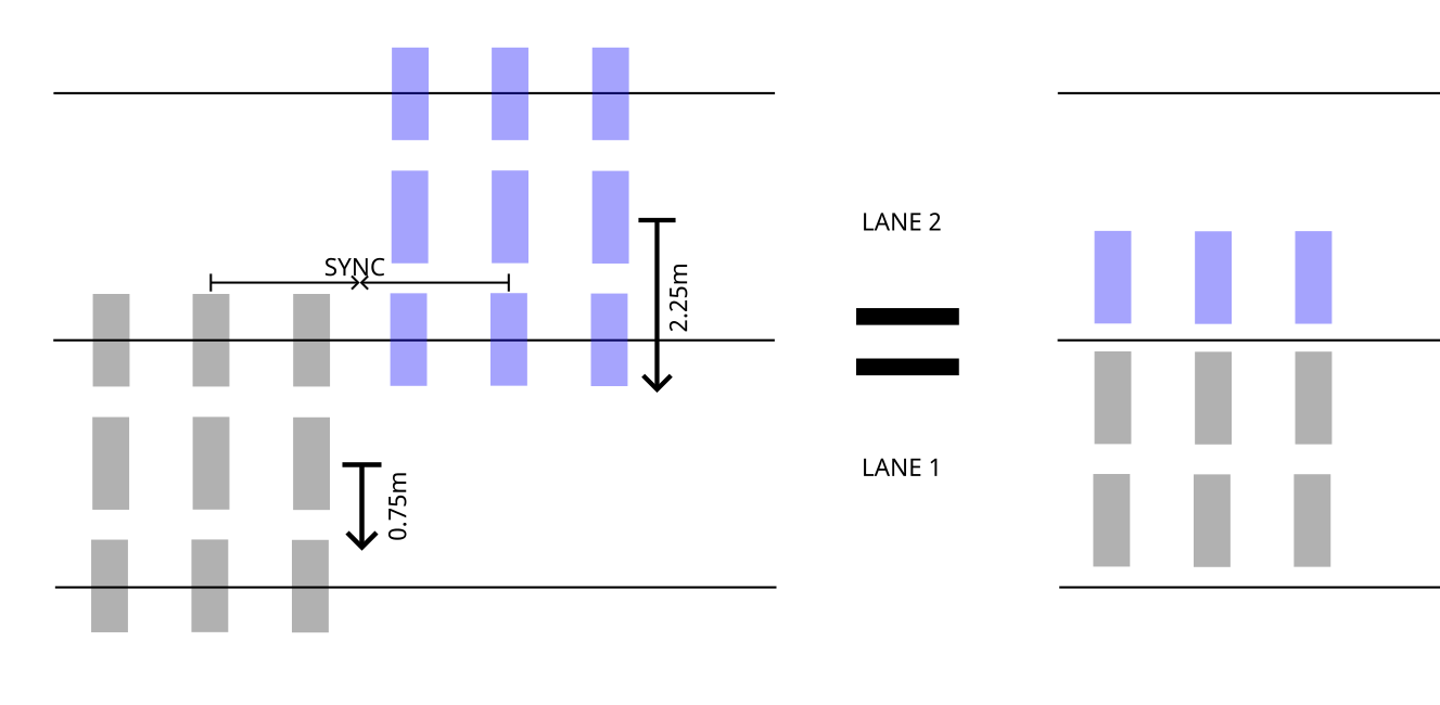
Here we apply the LM3 in both lanes that are covered by the special vehicle and shift the load trains in cross-direction (YEX) such that their positions match (and match with the specification of the code). Note that the loads of a lane that are not positioned within the lane are clipped. Therefore the loads are not applied twice, although we have used two load trains!
Finally we synchronize the load trains in longitudinal direction (SYNC) to make sure that the special vehicle that we have built from the two load trains moves as one instance.
Note
In the present example we have defined and used two load trains for the LM3, because in the first lane we have a different accompanying load train (LM1, frequent values of TS with axle load 300 kN; UDL loads of 9kN/m2) than in the second lane (LM1, frequent values of TS with axle load 200 kN; UDL loads of 2.5kN/m2)
Note
The shift in cross-direction with YEX is currently not displayed in the visualization window!